Lagrangian Formulation: 2R Planar Robot Example
This example demonstrates deriving the equations of motion for a 2R planar robot using the Lagrangian method, based on the setup from Modern Robotics.
The Problem Setup
We’re working with the 2R planar open chain robot shown below, acting under gravity.
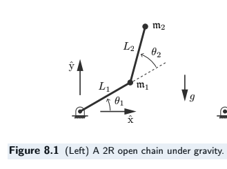
(Image based on Modern Robotics, Lynch & Park)
It’s simplified to represent a system with two point masses, \(m_1\) and \(m_2\), located at the distal ends of massless links of length \(L_1\) and \(L_2\), respectively. Gravity, with acceleration \(g\), acts in the negative \(\hat{y}_0\) direction (downwards in the base frame). The joint angles are \(\theta_1\) and \(\theta_2\).
Lagrangian Formulation Approach
Recalling Lagrangian Dynamics, the principle we use leverages the energy in the system (kinetic and potential) to determine the generalized forces (in this case, the joint torques) required for a given motion.
The core components are the Kinetic Energy (\(T\)) and Potential Energy (\(V\)) of the system.
Kinetic Energy (\(T\))
The kinetic energy of a rigid body \(i\) is generally: \(T_i = \frac{1}{2} m_i v_i^{2} + \frac{1}{2} I_i \omega_i^{2}\) (Where \(v_i\) is linear velocity, \(\omega_i\) is angular velocity, and \(I_i\) is the moment of inertia).
Given we are dealing with point masses located at the ends of the links, the rotational inertia term (\(I_i\)) is negligible because there is no mass distribution around the center of mass to create a moment of inertia about that point. Thus, the kinetic energy for each point mass simplifies to:
\[T_i = \frac{1}{2} m_i v_i^{2}\]The total kinetic energy of the system is the sum of the kinetic energies of each mass: \(T = T_1 + T_2\). We need to find the squared linear velocities (\(v_1^2\) and \(v_2^2\)) in terms of the joint angles and velocities.
Velocity of Mass 1 (\(v_1\))
The position of the first mass (\(m_1\)) is:
- \[x_1 = L_1 \cos(\theta_1)\]
- \[y_1 = L_1 \sin(\theta_1)\]
Taking the time derivatives gives the velocity components:
- \[\dot{x}_1 = - L_1 \sin(\theta_1) \dot{\theta_1}\]
- \[\dot{y}_1 = L_1 \cos(\theta_1) \dot{\theta_1}\]
The squared speed is:
\[v_1^2 = \dot{x}_1^2 + \dot{y}_1^2\]Using the identity \(\sin^2(\theta) + \cos^2(\theta) = 1\), this simplifies to:
\[v_1^2 = (-L_1 \sin(\theta_1) \dot{\theta_1})^2 + (L_1 \cos(\theta_1) \dot{\theta_1})^2 = L_1^2 \dot{\theta_1}^2\]So, the kinetic energy of the first mass is:
\[T_1 = \frac{1}{2} m_1 v_1^{2} = \frac{1}{2} m_1 L_1^2 \dot{\theta_1}^2\]Velocity of Mass 2 (\(v_2\))
The position of the second mass (\(m_2\), the end-effector) is:
\[x_2 = L_1 \cos(\theta_1) + L_2 \cos(\theta_1 + \theta_2)\] \[y_2 = L_1 \sin(\theta_1) + L_2 \sin(\theta_1 + \theta_2)\]Performing a time derivative gives the velocity components:
\[\dot{x}_2 = -L_1 \sin(\theta_1) \dot{\theta_1} - L_2 \sin(\theta_1 + \theta_2) (\dot{\theta_1} + \dot{\theta_2})\] \[\dot{y}_2 = L_1 \cos(\theta_1) \dot{\theta_1} + L_2 \cos(\theta_1 + \theta_2) (\dot{\theta_1} + \dot{\theta_2})\]Calculating the squared speed \(v_2^2 = \dot{x}_2^2 + \dot{y}_2^2\) involves significant algebraic simplification. The result is:
\[v_2^2 = (L_{1}^{2}+2L_{1}L_{2}\cos\theta_{2}+L_{2}^{2})\dot{\theta}_{1}^{2}+2(L_{2}^{2}+L_{1}L_{2}\cos\theta_{2})\dot{\theta}_{1}\dot{\theta}_{2}+L_{2}^{2}\dot{\theta}_{2}^{2}\]So, the kinetic energy of the second mass is:
\[T_2 = \frac{1}{2} m_2 v_2^{2} = \frac{1}{2} m_{2}((L_{1}^{2}+2L_{1}L_{2}\cos\theta_{2}+L_{2}^{2})\dot{\theta}_{1}^{2}+2(L_{2}^{2}+L_{1}L_{2}\cos\theta_{2})\dot{\theta}_{1}\dot{\theta}_{2}+L_{2}^{2}\dot{\theta}_{2}^{2})\]Total Kinetic Energy (\(T\))
The total kinetic energy is \(T = T_1 + T_2\).
Potential Energy (\(V\))
Given gravity acts in the \(- \hat{y}_0\) direction, the potential energy of each mass is \(V_i = m_i g y_i\), where \(y_i\) is the height of the mass.
-
Potential Energy of Mass 1 (\(V_1\)):
\[V_1 = m_1 g y_1 = m_1 g L_1 \sin(\theta_1)\] -
Potential Energy of Mass 2 (\(V_2\)):
\[V_2 = m_2 g y_2 = m_2 g (L_1 \sin(\theta_1) + L_2 \sin(\theta_1 + \theta_2))\] -
Total Potential Energy (\(V\)):
\(V = V_1 + V_2 = g (m_1 L_1 \sin(\theta_1) + m_2 (L_1 \sin(\theta_1) + L_2 \sin(\theta_1 + \theta_2)))\) \(V = g ((m_1 + m_2) L_1 \sin(\theta_1) + m_2 L_2 \sin(\theta_1 + \theta_2))\)
The Lagrangian (\(L\))
Now we can write the Lagrangian for the entire system:
\[L = T - V = (T_1 + T_2) - (V_1 + V_2)\]To find the rate of change of the energy in the system for infinitesimal changes in joint velocities and angles, we view the Lagrangian as a function of the independent generalized coordinates (\(\theta_1, \theta_2\)) and their velocities (\(\dot{\theta}_1, \dot{\theta}_2\)):
\[L(\theta_1, \theta_2, \dot{\theta_1}, \dot{\theta_2}) = T(\theta_2, \dot{\theta_1}, \dot{\theta_2}) - V(\theta_1, \theta_2)\]Equations of Motion via Euler-Lagrange
The equations of motion are found by applying the Euler-Lagrange equation for each joint angle. The general form is: \(\tau_i = \frac{d}{dt}\left(\frac{\partial L}{\partial\dot{\theta_i}}\right) - \frac{\partial L}{\partial\theta_i}\) Here, \(\tau_i\)represents the external torque applied at joint\(i\).
Calculating the necessary partial derivatives (\(\partial L / \partial \dot{\theta}_1\), \(\partial L / \partial \theta_1\), etc.) and the time derivatives (\(\frac{d}{dt}(...)\)) is algebraically intensive. Performing these steps leads to the following equations of motion:
Considering Joint 1 (\(\theta_1\)):
\[\begin{align*} \\ \tau_1 &= \frac{d}{dt}\left(\frac{\partial L}{\partial\dot{\theta_1}}\right) - \frac{\partial L}{\partial\theta_1} \\ &= (m_{1}L_{1}^{2}+m_{2}(L_{1}^{2}+2L_{1}L_{2}\cos\theta_{2}+L_{2}^{2}))\ddot{\theta}_{1} \\ &\quad +m_{2}(L_{1}L_{2}\cos\theta_{2}+L_{2}^{2})\ddot{\theta}_{2}-m_{2}L_{1}L_{2}\sin\theta_{2}(2\dot{\theta}_{1}\dot{\theta}_{2}+\dot{\theta}_{2}^{2}) \\ &\quad +(m_{1}+m_{2})L_{1}g\cos\theta_{1}+m_{2}gL_{2}\cos(\theta_{1}+\theta_{2}) \end{align*}\]Considering Joint 2 (\(\theta_2\)):
\[\begin{align*} \\ \tau_2 &= \frac{d}{dt}\left(\frac{\partial L}{\partial\dot{\theta_2}}\right) - \frac{\partial L}{\partial\theta_2} \\ &= m_{2}(L_{1}L_{2}\cos\theta_{2}+L_{2}^{2})\ddot{\theta}_{1}+m_{2}L_{2}^{2}\ddot{\theta}_{2}+m_{2}L_{1}L_{2}\dot{\theta}_{1}^{2}\sin\theta_{2} \\ &\quad +m_{2}gL_{2}\cos(\theta_{1}+\theta_{2}) \end{align*}\]Standard Manipulator Equation Form
The two complex equations for \(\tau_1\) and \(\tau_2\) derived from the Euler-Lagrange method can be organized into a standard matrix form used widely in robotics:
\[M(\theta)\ddot{\theta} + C(\theta, \dot{\theta})\dot{\theta} + G(\theta) = \tau\]Here’s how the terms group together:
- \(\tau = [\tau_1, \tau_2]^T\): The vector of external torques applied at each joint (our inputs or outputs depending on the problem).
-
\(\theta = [\theta_1, \theta_2]^T\): The vector of joint angles. Correspondingly, \(\dot{\theta}\)and\(\ddot{\theta}\) are the vectors of joint velocities and accelerations.
- \(M(\theta)\): The Mass Matrix (or Inertia Matrix). This is a \(2 \times 2\) matrix containing all the terms that multiply the joint accelerations (\(\ddot{\theta}_1\) and \(\ddot{\theta}_2\)). It depends on the current configuration \(\theta\) (specifically \(\theta_2\) in this case) and describes the system’s resistance to acceleration.
- \(C(\theta, \dot{\theta})\dot{\theta}\): The vector of Coriolis and Centrifugal Torques. These terms arise naturally from differentiating the kinetic energy (which contains velocity products and squares) within the Euler-Lagrange framework, even for point masses moving in rotating frames. They depend on both joint positions \(\theta\) and velocities \(\dot{\theta}\).
- Centrifugal terms: Proportional to \(\dot{\theta}_i^2\).
- Coriolis terms: Proportional to \(\dot{\theta}_i \dot{\theta}_j\). For our system, this vector collects terms like \(-m_{2}L_{1}L_{2}\sin\theta_{2}(2\dot{\theta}_{1}\dot{\theta}_{2}+\dot{\theta}_{2}^{2})\) and \(m_{2}L_{1}L_{2}\dot{\theta}_{1}^{2}\sin\theta_{2}\).
- \(G(\theta)\): The vector of Gravitational Torques. These terms come from differentiating the potential energy \(V\)with respect to the joint angles \(\theta\) (specifically the \(\frac{\partial L}{\partial \theta_i}\)part of the Euler-Lagrange equation). They depend only on the configuration \(\theta\).
Forward Dynamics
This standard form clearly separates the influences on the robot’s motion. A common task is forward dynamics: calculating the resulting joint accelerations (\(\ddot{\theta}\)) given the current state (\(\theta, \dot{\theta}\)) and the applied torques (\(\tau\)). To do this, we rearrange the equation to isolate \(\ddot{\theta}\):
\[M(\theta)\ddot{\theta} = \tau - (C(\theta, \dot{\theta})\dot{\theta} + G(\theta))\]For convenience, often all the velocity- and position-dependent forces (Coriolis, centrifugal, gravity) are grouped into a single vector function \(h(\theta, \dot{\theta})\):
\[h(\theta, \dot{\theta}) \equiv C(\theta, \dot{\theta})\dot{\theta} + G(\theta)\]Substituting this definition gives the compact form:
\[M(\theta)\ddot{\theta} = \tau - h(\theta, \dot{\theta})\]We can now solve for the unknown joint accelerations, \(\ddot{\theta}\), by inverting the mass matrix (which is always possible for physical systems):
\[\ddot{\theta} = M(\theta)^{-1}(\tau - h(\theta, \dot{\theta}))\]This final equation is the core of simulating the robot’s motion forward in time. Given the current state and motor commands, it tells you how the robot will accelerate.
Credit: Example setup and equations adapted from “Modern Robotics: Mechanics, Planning, and Control” by Lynch and Park, Chapter 8.