The Robot Used For This Forward Kinematics Study: UR5
The robot consists of 6 revolute joints (6R)
The key elements to model the Forward Kinematics (F.K) are:
- Define the fixed base frame \(\{s\}/\{0\}\) as the reference coordinate system.
- Specify the home position of the end-effector.
- Define the screw axes for each joint.
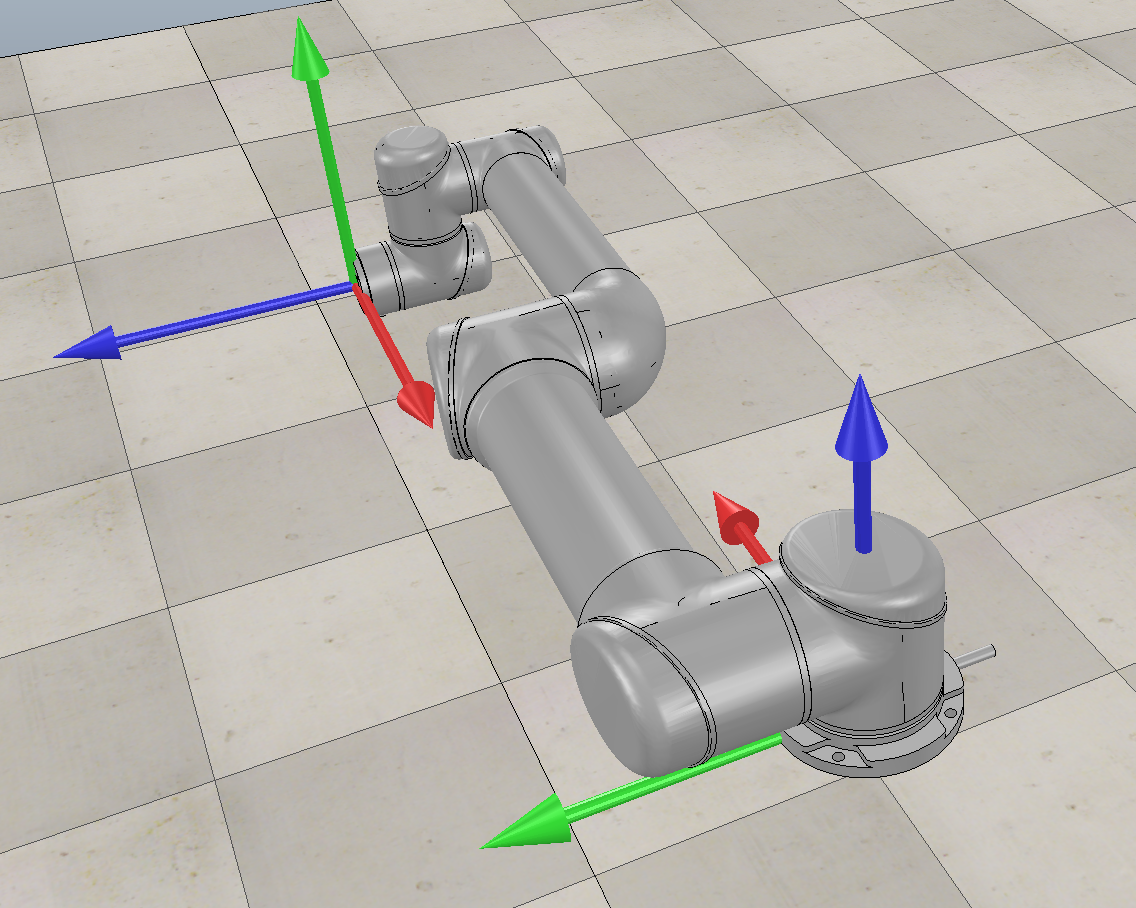
Fixed frame:
We take the robot’s base as the fixed frame \(\{s\}\), which follows a right-handed coordinate system.
End-effector home position in the fixed frame:
- The matrix \(M\) encodes the position and orientation of the end-effector at the home position.
- The local coordinate axes of the end-effector relate to the fixed frame axes as follows:
- The local \(x\)-axis is anti-parallel to the fixed frame’s \(x\)-axis.
- The local \(y\)-axis is aligned with the fixed frame’s \(z\)-axis.
- The local \(z\)-axis is aligned with the fixed frame’s \(y\)-axis.
The end-effector local axis position represented in the fixed frame,
\[p = \begin{bmatrix} L1+L2 \\ W1+W2 \\ H1-H2\\ \end{bmatrix}\]We combine the position and orientation into a homogeneous transformation matrix
\[M = \begin{bmatrix} R_{0,6} & p_{0,6} \\ \mathbf{0}_{1 \times 3} & 1 \\ \end{bmatrix} = \begin{bmatrix} -1 & 0 & 0 & L1+L2 \\ 0 & 0 & 1 & W1+W2 \\ 0 & 1 & 0 & H1-H2\\ 0 & 0 & 0 & 1\\ \end{bmatrix}\]Determining the screw axes:
The general form of the screw axis is comprised of angular velocity \(\vec{\omega}\) and instantaneous velocity \(\vec{v}\), where
\[\vec{v} = - \vec{\omega} \times \vec{q}\]where:
- \(\vec{\omega}\) is the unit vector along the axis of rotation (angular velocity direction).
- \(\vec{q}\) is a point on the axis of rotation.
Note:
If the point \(\vec{p}\) is not on the rotation axis, then the shortest distance vector from \(\vec{p}\) to the axis, given by \((\vec{p} - \vec{q})\), is used to calculate the linear velocity:
| Joint | Angular Velocity | Instantaneous Velocity | Screw Axis |
|---|---|---|---|
| S1 | $$ \begin{bmatrix} 0 \\ 0 \\ 1 \\ \end{bmatrix} $$ | $$ \begin{bmatrix} 0 \\ 0 \\ 0 \\ \end{bmatrix} $$ | $$ \begin{bmatrix} 0 \\ 0 \\ 1 \\ 0 \\ 0 \\ 0 \\ \end{bmatrix} $$ |
| S2 | $$ \begin{bmatrix} 0 \\ 1 \\ 0 \\ \end{bmatrix} $$ | $$ \begin{bmatrix} -H_1 \\ 0 \\ 0 \\ \end{bmatrix} $$ | $$ \begin{bmatrix} 0 \\ 1 \\ 0 \\ -H_1 \\ 0 \\ 0 \\ \end{bmatrix} $$ |
| S3 | $$ \begin{bmatrix} 0 \\ 1 \\ 0 \\ \end{bmatrix} $$ | $$ \begin{bmatrix} -H_1 \\ 0 \\ L_1 \\ \end{bmatrix} $$ | $$ \begin{bmatrix} 0 \\ 1 \\ 0 \\ -H_1 \\ 0 \\ L_1 \\ \end{bmatrix} $$ |
| S4 | $$ \begin{bmatrix} 0 \\ 1 \\ 0 \\ \end{bmatrix} $$ | $$ \begin{bmatrix} -H_1 \\ 0 \\ L_1 + L_2 \\ \end{bmatrix} $$ | $$ \begin{bmatrix} 0 \\ 1 \\ 0 \\ -H_1 \\ 0 \\ L_1 + L_2 \\ \end{bmatrix} $$ |
| S5 | $$ \begin{bmatrix} 0 \\ 0 \\ -1 \\ \end{bmatrix} $$ | $$ \begin{bmatrix} -W_1 \\ L_1 + L_2 \\ 0 \\ \end{bmatrix} $$ | $$ \begin{bmatrix} 0 \\ 0 \\ -1 \\ -W_1 \\ L_1 + L_2 \\ 0 \\ \end{bmatrix} $$ |
| S6 | $$ \begin{bmatrix} 0 \\ 1 \\ 0 \\ \end{bmatrix} $$ | $$ \begin{bmatrix} H_2 - H_1 \\ 0 \\ L_1 + L_2 \\ \end{bmatrix} $$ | $$ \begin{bmatrix} 0 \\ 1 \\ 0 \\ H_2 - H_1 \\ 0 \\ L_1 + L_2 \\ \end{bmatrix} $$ |
To represent the screw axis in homogeneous coordinates,
the angular velocity vector \(\mathbf{w}\) is expressed using its skew-symmetric matrix form. This matrix is then augmented with an additional row and column \([0 \quad 0 \quad 0 \quad 1]\) to construct a \(4 \times 4\) matrix. This representation enables smooth matrix operations within the homogeneous transformation framework.
\[\begin{bmatrix} [w] & v_i \\ \mathbf{0}_{1 \times 3} & 1 \\ \end{bmatrix}\]Mathematical model for Forward Kinematics of open chain
The forward kinematics of the chain is given by the screw axis of each joint, the corresponding joint angles, and the home configuation of the end effector.
This is expressed using the Product of Exponentials (PoE) representation:
\[T = e^{[S_1] \cdot \theta_1} \cdot e^{[S_2] \cdot \theta_2} \cdot e^{[S_3] \cdot \theta_3} \cdot e^{[S_4] \cdot \theta_4} \cdot e^{[S_5] \cdot \theta_5} \cdot e^{[S_6] \cdot \theta_6} \cdot M\]Note:
- The general form of the matrix exponential \(e^{[\vec{\omega}] \theta}\) is given by the Rodrigues formula:
where \(I\) is the identity matrix, and \([\vec{\omega}]\) is the skew-symmetric matrix corresponding to the unit vector \(\vec{\omega}\).
- Given a unit vector \(\vec{\omega} \in \mathbb{R}^3\) and a scalar \(\theta\), the matrix exponential satisfies:
- For the zero matrix exponent, we have:
\(e^{0} = I\) —
Time to Validate
I have used CoppeliaSim tool with the UR5 model to verify the assumptions.
The joint angles used in the simulation were:
\[\theta_{\text{vals}} = [0, -1.73, 0.811, -1.292, -1.232, 1.953]\]For the above joint angles, the computed SE(3) end-effector matrix (using Python) matches the simulated results:
\[T_{\text{computed}} = \begin{bmatrix} -0.8182 & 0.1149 & 0.5634 & 0.2928 \\ 0.3518 & 0.8751 & 0.3324 & 0.1363 \\ -0.4548 & 0.4701 & -0.7564 & 0.8150 \\ 0 & 0 & 0 & 1.0000 \end{bmatrix}\]| Arm visual after applying joint angles | CoppeliaSim computed matrix |
|---|---|
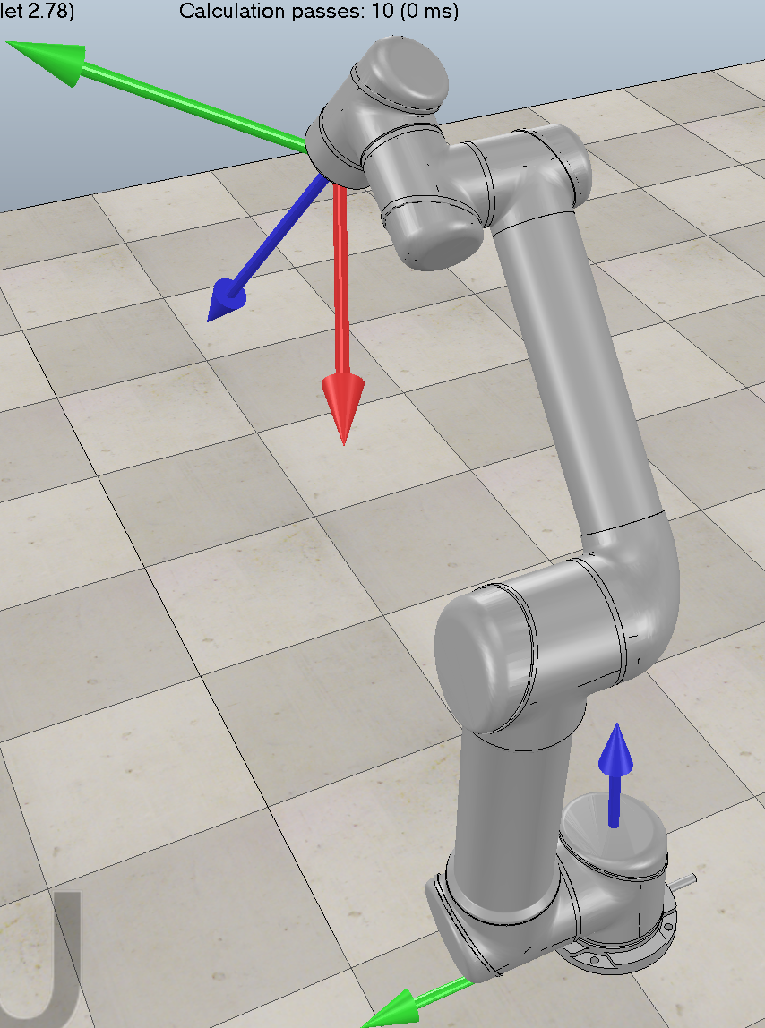 | 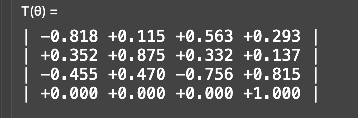 |
Note: This work is for educational purposes only. CoppeliaSim was used solely to perform simulations.