Taming Gravity: Implementing and Simulating UR5 Dynamics
This project documents the end-to-end process of deriving, implementing, and simulating a full dynamic model for a UR5 robot arm using Lagrangian dynamics. We begin from first principles, translate the mathematics into a robust software implementation, and validate the results in the CoppeliaSim (Evaluation version) physics-based simulator.
Motivation and Approach: From Theory to Application
The core physics is modeled using Lagrangian Dynamics, leveraging the principles discussed in our theory sections on Lagrangian Dynamics and the Calculus of Variation, to derive the equations of motion from the system’s energy.
While the elegant Product of Exponentials (PoE) and screw axis theory (as described in Modern Robotics by Lynch and Park) is a great choice for kinematics, this project takes a deliberate detour using the classic Denavit-Hartenberg (DH) parameters.
Why DH? As a foundational exercise to build a strong intuition for 3D geometric projections. The process of implementing a DH calculator was a challenging but rewarding journey that involved:
- Visualization of coordinate frames
- Axis projections
- Traversing the kinematic chain following the 4-step recipe to find the parameters:
- \(a\):
_get_link_length - \(\alpha\):
_get_link_twist - \(d\):
_get_link_offset - \(\theta\):
_get_joint_angle
- \(a\):
Software Architecture: A Modular Approach
The codebase is built on a foundation of SOLID principles and design patterns, ensuring it is modular, maintainable, extensible and testable.
The dynamics simulation involves several key modules:
A central WorkflowFacade that orchestrates the entire process, delegating tasks to specialized, swappable modules based on strategy patterns.
- Forward Kinematics Module: Responsible for calculating the robot’s forward kinematics. It supports multiple strategies:
- Denavit-Hartenberg
- Product-of-Exponentials
For this workflow run, the
Denavit-Hartenbergstrategy is used, injected with the custom-built DH calculator. - Dynamics Module: Derives the equations of motion. This module also supports multiple strategies:
- Lagrangian formulation
- Newton–Euler formulation
For this workflow run, we use the
Lagrangian Dynamicsformulation strategy. Its key operations include:- Symbolically deriving the full equations of motion using Python’s
sympy/scipylibrary. - Extracting the dynamic matrices:
- Mass Matrix (\(M(q)\))
- Coriolis/Centrifugal Matrix (\(C(q, \dot{q})\))
- Gravity Vector (\(G(q)\)).
- (Inverse Dynamics calculation is planned for future implementation).
- Simulation Controller: Orchestrates different simulation scenarios by interacting with the Dynamics Module and the Simulation Connector. Supports various control strategies, for example, the
GravityCompensationControllerimplemented for this validation, which reads the robot’s state and applies the calculated gravity torques. - Simulation Connector: Developed a reusable, abstracted connector for CoppeliaSim (Evaluation version) using well-defined contracts for cross-project compatibility. Handles fetching model data (joint configurations, mass properties) and executing commands within the simulation loop. Employed Test-Driven Development (TDD) when adding features to the connectors, such as applying joint torque, to ensure robustness against API changes and maintain generic method design.
Miscellaneous
- Data Handling: Data Transfer Objects (DTOs) and Enums are used throughout to ensure clean data encapsulation (e.g., FK chains, transformation matrices, COMs, rotation axes, symbolic variables) and provide a unified, type-safe way to access robot model components in the pipeline.
- Audit and Debugging: All intermediate mathematical steps (symbolic computations) are logged to files, which proved invaluable for verification and debugging.
- Efficiency: A read-through caching strategy saves the results of expensive symbolic computations (like dynamic matrices, DH parameters and the FK transformation matrices) to file. This significantly speeds up subsequent runs during development, debugging, and analysis.
The Goal: Validating the Gravity Compensation (\(G(q)\))
The primary goal of this simulation is to validate our derived mathematical model. Specifically, we want to confirm that our symbolically computed Gravity Vector (\(G(q)\)) accurately represents the torques required to counteract gravity within the physics simulation for the UR5.
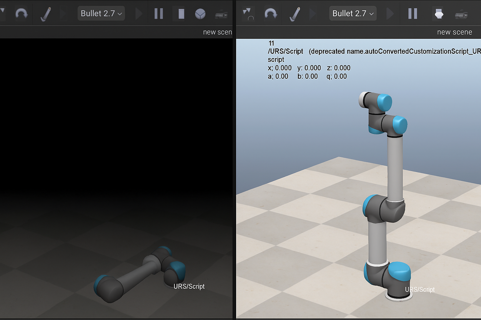
We test this by running two scenarios in CoppeliaSim, starting from the robot’s home configuration:
-
Scenario 1: No Gravity Compensation (Apply Zero Torques): The controller commands zero torque (\(\tau = \mathbf{0}\)) to all joints. As expected, the simulated robot arm will collapse under its own weight, as there are no torques to hold it in position.
-
Scenario 2: Apply Computed Gravity Compensation Torques: The controller calculates the Gravity Vector \(G(q)\) based on the robot’s current joint configuration \(q\) using our derived model. The resulting torques are applied directly in joint space, without feedback control. The controller commands joint torques equal to this vector (\(\tau = G(q)\)) to the joints. If our model is accurate, these torques should perfectly counteract the force of gravity at every joint. With no other external forces acting on the system, the arm should maintain its position, effectively appearing weightless.
Simulation Results: Taming Gravity in Action
With the mathematical model derived and the software architecture in place, we proceed to the validation stage in CoppeliaSim. The following sections present the results of our two test scenarios.
The Execution Flow
The first time the application runs, it performs a full symbolic derivation of the robot’s dynamics. This is a computationally intensive, one-time process. The logs below capture the key stages of this initial run.
Initial Derivation Log Snippet:
[INFO] --- Cache file not found. Running full symbolic derivation.
[INFO] --- --- Calculating Forward Kinematics using Denavit-Hartenberg ---
[INFO] --- Calculating DH for link between BASE and JOINT_1
[INFO] ---   Stored FK data for J1
... (FK calculations for J2-J5 omitted for brevity) ...
[INFO] --- Calculating DH for link between JOINT_5 and JOINT_6
[INFO] ---   Stored FK data for J6
[INFO] --- --- Deriving Equations of Motion using Lagrangian Method---
[INFO] --- Deriving equation for Joint 1 (tau_1)
... (EOM derivations for J2-J5 omitted for brevity) ...
[INFO] --- Deriving equation for Joint 6 (tau_6)
[INFO] --- Successfully derived all equations of motion.
[INFO] --- --- Extracting Dynamic Matrices (M, C, G) ---
[INFO] --- Finished extracting M, C, and G.
[INFO] --- Dumping data to pickle cache file: dynamic_matrices.pkl
Using the Cache on Subsequent Runs: On subsequent runs, the system loads the pre-computed functions, significantly speeding up initialization:
[INFO] --- Loading dynamic matrices from cache file: dynamic_matrices.pkl
[INFO] --- --- Preparing Forward Dynamics Simulator ---
This read-through caching strategy is for efficient development and testing.
Scenario 1: No Gravity Compensation (The Fall)
In this test, the joint torques are set to zero (\(\tau = \mathbf{0}\)). As the physics simulation starts, the robot arm has no forces to counteract gravity and collapses under its own weight.
Zero Torque Log Snippets:
[INFO] --- --- Starting DYNAMIC Simulation Loop (Zero Torque) ---
[INFO] --- All joints set to torque/force mode.
[INFO] --- t= 0.00s | Pos: [ J1:   -0.0° | J2:   -0.0° | J3:   -0.0° | J4:   -0.0° | J5:    0.0° | J6:    0.0° ]
[INFO] ---           | Applied:  [ Cmd_τ1:    0.0 | Cmd_τ2:    0.0 | Cmd_τ3:    0.0 | Cmd_τ4:    0.0 | Cmd_τ5:    0.0 | Cmd_τ6:    0.0 ]
[INFO] ---           | Measured: [ Meas_τ1:    0.0 | Meas_τ2:    0.0 | Meas_τ3:    0.0 | Meas_τ4:    0.0 | Meas_τ5:    0.0 | Meas_τ6:    0.0 ]

[INFO] --- t= 1.00s | Pos: [ J1:  -19.3° | J2:  -91.9° | J3:  164.7° | J4: -187.5° | J5:   68.2° | J6:   99.7° ]
[INFO] ---           | Applied:  [ Cmd_τ1:    0.0 | Cmd_τ2:    0.0 | Cmd_τ3:    0.0 | Cmd_τ4:    0.0 | Cmd_τ5:    0.0 | Cmd_τ6:    0.0 ]
[INFO] ---           | Measured: [ Meas_τ1:    0.0 | Meas_τ2:    0.0 | Meas_τ3:    0.0 | Meas_τ4:    0.0 | Meas_τ5:    0.0 | Meas_τ6:    0.0 ]

[INFO] --- t= 4.00s | Pos: [ J1:  -19.3° | J2:  -91.9° | J3:  164.7° | J4: -187.5° | J5:   54.7° | J6:   96.9° ]
[INFO] ---           | Applied:  [ Cmd_τ1:    0.0 | Cmd_τ2:    0.0 | Cmd_τ3:    0.0 | Cmd_τ4:    0.0 | Cmd_τ5:    0.0 | Cmd_τ6:    0.0 ]
[INFO] ---           | Measured: [ Meas_τ1:    0.0 | Meas_τ2:    0.0 | Meas_τ3:    0.0 | Meas_τ4:    0.0 | Meas_τ5:    0.0 | Meas_τ6:    0.0 ]
[INFO] --- --- DYNAMIC Simulation Loop Finished ---
These logs clearly show the joint positions changing dramatically from the initial zero state within the first second and continuing to drift, confirming the arm collapses when no compensating torque is applied.
Scenario 2: Gravity Compensation Enabled (The Stable Hold)
Here, In each simulation step, the controller:
- Reads the current joint angles \(q\).
- Calculates the required gravity-compensating torques using our derived function: \(\tau_{cmd} = G(q)\).
- Applies these torques to the corresponding joints.
The result is a stable robot that holds its position, appearing weightless as our controller perfectly “tames” the force of gravity.
Gravity Compensation Log Snippets:
[INFO] --- All joints set to torque/force mode.
[INFO] --- t= 0.00s | Pos: [ J1:   -0.0° | J2:   -0.0° | J3:   -0.0° | J4:   -0.0° | J5:    0.0° | J6:    0.0° ]
[INFO] ---           | Applied:  [ Cmd_τ1:   -0.0 | Cmd_τ2: -100.5 | Cmd_τ3:  -36.7 | Cmd_τ4:   -0.0 | Cmd_τ5:   -0.0 | Cmd_τ6:   -0.0 ]
[INFO] ---           | Measured: [ Meas_τ1:    0.0 | Meas_τ2:   -0.0 | Meas_τ3:    0.0 | Meas_τ4:   -0.0 | Meas_τ5:   -0.0 | Meas_τ6:    0.0 ]
[INFO] --- t= 1.00s | Pos: [ J1:   -0.0° | J2:   -0.0° | J3:    0.0° | J4:   -0.0° | J5:    0.0° | J6:   -0.0° ]
[INFO] ---           | Applied:  [ Cmd_τ1:   -0.0 | Cmd_τ2: -100.5 | Cmd_τ3:  -36.7 | Cmd_τ4:   -0.0 | Cmd_τ5:   -0.0 | Cmd_τ6:   -0.0 ]
[INFO] ---           | Measured: [ Meas_τ1:    0.0 | Meas_τ2:   -0.0 | Meas_τ3:    0.0 | Meas_τ4:   -0.0 | Meas_τ5:    0.0 | Meas_τ6:    0.0 ]
[INFO] --- t= 2.00s | Pos: [ J1:   -0.0° | J2:   -0.0° | J3:    0.0° | J4:   -0.0° | J5:    0.0° | J6:   -0.0° ]
[INFO] ---           | Applied:  [ Cmd_τ1:   -0.0 | Cmd_τ2: -100.5 | Cmd_τ3:  -36.7 | Cmd_τ4:   -0.0 | Cmd_τ5:   -0.0 | Cmd_τ6:   -0.0 ]
[INFO] ---           | Measured: [ Meas_τ1:    0.0 | Meas_τ2:   -0.0 | Meas_τ3:    0.0 | Meas_τ4:   -0.0 | Meas_τ5:    0.0 | Meas_τ6:    0.0 ]
[INFO] --- t= 3.00s | Pos: [ J1:   -0.0° | J2:   -0.0° | J3:    0.0° | J4:   -0.0° | J5:    0.0° | J6:   -0.1° ]
[INFO] ---           | Applied:  [ Cmd_τ1:   -0.0 | Cmd_τ2: -100.5 | Cmd_τ3:  -36.7 | Cmd_τ4:   -0.0 | Cmd_τ5:   -0.0 | Cmd_τ6:   -0.0 ]
[INFO] ---           | Measured: [ Meas_τ1:    0.0 | Meas_τ2:   -0.0 | Meas_τ3:    0.0 | Meas_τ4:   -0.0 | Meas_τ5:    0.0 | Meas_τ6:    0.0 ]
[INFO] --- t= 4.00s | Pos: [ J1:   -0.0° | J2:   -0.0° | J3:    0.0° | J4:   -0.0° | J5:    0.0° | J6:   -0.1° ]
[INFO] ---           | Applied:  [ Cmd_τ1:   -0.0 | Cmd_τ2: -100.5 | Cmd_τ3:  -36.7 | Cmd_τ4:   -0.0 | Cmd_τ5:   -0.0 | Cmd_τ6:   -0.0 ]
[INFO] ---           | Measured: [ Meas_τ1:    0.0 | Meas_τ2:   -0.0 | Meas_τ3:    0.0 | Meas_τ4:   -0.0 | Meas_τ5:    0.0 | Meas_τ6:    0.0 ]
[INFO] --- --- DYNAMIC Simulation Loop Finished ---
These logs clearly show the joint positions are maintained stably around their initial zero values, validating that the associated applied torques calculated from our \(G(q)\) model are successfully counteracting and therefore “taming” the force of gravity.